1. 项目准备
1.1. 问题导入
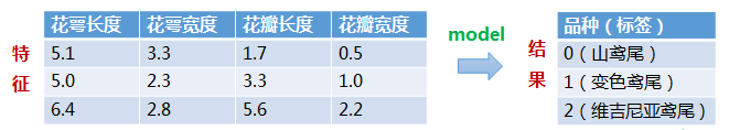
构建一个模型,根据鸢尾花的花萼大小和花瓣大小将其分为三种不同的品种:
1.2. 数据集简介
数据集共包含150行数据,每一行数据由四个特征值及一个目标值组成。
这是数据集的下载链接:鸢尾花数据集 - AI Studio
2. 实验步骤
2.0.导入模块
1
2
3
4
5
import numpy as npfrom sklearn import svmfrom sklearn.model_selection import train_test_splitfrom matplotlib.colors import ListedColormapimport matplotlib.pyplot as plt
2.1. 数据准备
1
2
3
4
5
6
7
def iris_type (s ): it = { b'Iris-setosa' : 0 , b'Iris-versicolor' : 1 , b'Iris-virginica' : 2 } return it[s]
1
2
3
4
5
6
7
data_path = 'iris.data' data = np.loadtxt( data_path, dtype=float , delimiter=',' , converters={4 : iris_type} )
1
2
3
4
5
6
x, y = np.split( data, (4 , ), axis=1 ) x = x[:, 0 :2 ]
1
2
3
4
5
6
x_train, x_test, y_train, y_test = train_test_split( x, y, random_state=1 , test_size=0.3 )
2.2. 模型搭建
C值大,对误分类的惩罚增大,这样趋向于训练集测试的准确率很高,但泛化能力弱
C值小,对误分类的惩罚减小,允许容错,泛化能力较强
“linear”代表“线性核”,“rbf”代表“高斯核”。
gamma是选择rbf函数作为kernel后,该函数的一个参数,它隐含地决定了数据映射到新的特征空间后的分布。
gamma越小,分类界面越连续;gamma越大,分类界面越“散”,分类效果越好,但可能过拟合。
划分方法 decision_function_shape
“ovr”代表“one v rest”,即一个类别与其他类别进行划分;
“ovo”代表“one v one”,即将类别两两之间进行划分,用二分类的方法模拟多分类的结果。
1 2 3 4 clf = svm.SVC(C=0.5 , kernel='linear' , decision_function_shape='ovr' )
2.3. 模型训练
1
2
3
clf.fit(x_train, y_train.ravel())
2.4. 模型评估
1
2
3
def show_accuracy (a, b, tip ): acc = a.ravel() == b.ravel() print ("%s上的准确率 \t %.3f" % (tip, np.mean(acc)))
1
2
3
4
5
print ("训练集上的评分 \t %.3f" % clf.score(x_train, y_train))print ("测试集上的评分 \t %.3f" % clf.score(x_test, y_test))show_accuracy(clf.predict(x_train), y_train, "训练集" ) show_accuracy(clf.predict(x_test), y_test, "测试集" )
1
2
3
4
训练集上的评分 0.819 测试集上的评分 0.778 训练集上的准确率 0.819 测试集上的准确率 0.778
决策函数的值
1
2
3
4
values = clf.decision_function(x_train) print ("Iris-setosa \t Iris-versicolor \t Iris-virginica" )for lt in values: print ("%9.6f \t %9.6f \t\t %9.6f" % tuple (lt))
1
2
3
4
5
6
7
8
9
10
11
12
13
14
15
16
17
18
19
20
21
22
23
24
25
26
27
28
29
30
31
32
33
34
35
36
37
38
39
40
41
42
43
44
45
46
47
48
49
50
51
52
53
54
55
56
57
58
59
60
61
62
63
64
65
66
67
68
69
70
71
72
73
74
75
76
77
78
79
80
81
82
83
84
85
86
87
88
89
90
91
92
93
94
95
96
97
98
99
100
101
102
103
104
105
106
Iris-setosa Iris-versicolor Iris-virginica -0.500000 1.208873 2.291127 2.063288 -0.076968 1.013680 2.166750 0.917028 -0.083778 2.114278 0.997652 -0.111931 0.992554 2.063921 -0.056475 2.117430 0.952555 -0.069985 2.056150 -0.041847 0.985697 -0.318666 1.026860 2.291806 -0.271663 1.091503 2.180159 -0.378276 1.142604 2.235671 -0.221507 1.111050 2.110458 -0.183312 2.100667 1.082645 -0.054450 0.999278 2.055172 -0.469778 1.178538 2.291240 -0.057601 2.044375 1.013226 2.174723 0.936981 -0.111704 -0.133157 2.120214 1.012943 -0.217521 2.121026 1.096495 2.114278 0.997652 -0.111931 2.163598 0.962125 -0.125724 -0.210383 1.085906 2.124477 2.212918 0.926599 -0.139517 -0.133992 1.065140 2.068852 -0.180161 1.055570 2.124590 -0.233467 1.081121 2.152346 -0.087824 2.074710 1.013113 -0.203245 1.050785 2.152460 -0.114894 1.059949 2.054945 2.177874 -0.108116 0.930242 -0.235784 2.181291 1.054492 -0.206396 1.095882 2.110514 -0.210383 1.085906 2.124477 -0.029695 2.114210 0.915486 -0.126854 1.030020 2.096834 -0.094962 2.109831 0.985131 2.105470 -0.077374 0.971904 2.110292 0.987676 -0.097968 2.204110 -0.148428 0.944318 -0.203245 1.050785 2.152460 2.190669 0.976887 -0.167556 -0.160228 2.105452 1.054776 -0.236619 1.126218 2.110401 -0.095797 2.054758 1.041039 2.113443 -0.057421 0.943978 2.102319 0.967723 -0.070042 -0.122032 2.095070 1.026963 2.110292 0.987676 -0.097968 -0.412485 1.162964 2.249521 -0.168201 1.085499 2.082701 -0.420458 1.143011 2.277447 -0.248578 1.096288 2.152290 -0.277966 2.181698 1.096268 -0.092645 1.009660 2.082985 -0.253400 1.031238 2.222161 -0.053615 2.054351 0.999263 2.153955 -0.167975 1.014019 -0.122032 2.095070 1.026963 2.065793 1.088253 -0.154046 -0.110073 2.124999 0.985074 -0.271663 1.091503 2.180159 2.136527 0.947364 -0.083891 -0.297898 1.131815 2.166083 2.151639 0.932196 -0.083835 2.174723 0.936981 -0.111704 -0.111743 1.014852 2.096891 -0.068726 2.069519 0.999207 -0.237454 1.071144 2.166309 2.121416 0.962532 -0.083948 2.162763 -0.092948 0.930185 -0.065574 1.024422 2.041152 2.167585 0.972102 -0.139687 -0.122032 2.095070 1.026963 2.129389 0.982485 -0.111874 -0.210383 1.085906 2.124477 2.019625 1.078683 -0.098307 2.182696 0.956934 -0.139630 -0.161063 1.050379 2.110684 2.209767 0.971696 -0.181462 -0.038504 2.039183 0.999320 2.175558 0.992055 -0.167613 -0.110073 2.124999 0.985074 -0.075029 2.159713 0.915316 2.132541 0.937388 -0.069928 2.095180 1.002844 -0.098024 1.004513 2.093851 -0.098364 2.243141 0.896263 -0.139403 -0.095797 2.054758 1.041039 -0.149103 1.080308 2.068795 2.136527 0.947364 -0.083891 -0.233467 1.081121 2.152346 -0.072712 2.059543 1.013170 -0.273979 2.191674 1.082305 -0.275649 1.081527 2.194122 -0.122032 2.095070 1.026963 2.060137 -0.031871 0.971734 2.076083 1.008035 -0.084118 -0.194437 2.125811 1.068625 -0.164214 2.095476 1.068739 -0.344067 1.122245 2.221822 -0.118046 2.105046 1.013000 -0.202410 1.105859 2.096551 -0.176174 1.065547 2.110627 -0.247743 2.151362 1.096381 -0.233467 1.081121 2.152346 2.110292 0.987676 -0.097968
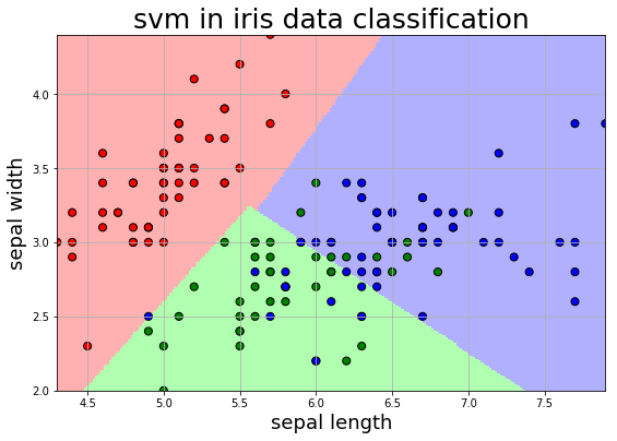
2.5. 可视化展示
1
2
3
4
5
6
7
x1_min, x1_max = x[:, 0 ].min (), x[:, 0 ].max () x2_min, x2_max = x[:, 1 ].min (), x[:, 1 ].max () x1, x2 = np.mgrid[x1_min:x1_max:200j , x2_min:x2_max:200j ] grid_test = np.stack((x1.flat, x2.flat), axis=1 ) z = clf.decision_function(grid_test) grid_hat = clf.predict(grid_test)
1 2 3 4 5 6 7 8 9 10 11 12 13 14 15 16 17 18 19 20 plt.figure(figsize=[9 , 6 ]) plt.title("svm in iris data classification" , fontsize=25 ) tags = ['sepal length' , 'sepal width' , 'petal length' , 'petal width' ] plt.xlabel(tags[0 ], fontsize=18 ) plt.ylabel(tags[1 ], fontsize=18 ) plt.xlim(x1_min, x1_max) plt.ylim(x2_min, x2_max) cm_light = ListedColormap(['#FFB0B0' , '#B0FFB0' , '#B0B0FF' ]) grid_hat = grid_hat.reshape(x1.shape) plt.pcolormesh(x1, x2, grid_hat, cmap=cm_light) cm_dark = ListedColormap(['red' , 'green' , 'blue' ]) plt.scatter(x[:, 0 ], x[:, 1 ], c=np.squeeze(y), edgecolor='k' , s=50 , cmap=cm_dark) plt.scatter(x_test[:, 0 ], x_test[:, 1 ], s=120 , facecolor="none" , zorder=10 ) plt.grid() plt.show()
写在最后